Steering Language Models and Interpretability

When a transformer-based LLM reads the text “The cat jumped on the table” how does it know you’re talking about the feline species of the animal kingdom and not something else? The model perceives everything in tokens, where each token typically corresponds to a word or subword (this is very nuanced and implementation dependent).

Example GPT 5 tokenization for this sentence

Each of these tokens gets mapped to a vector in the embedding matrix which makes up a subset of the model weights. These embedding vectors then activate features inside the model’s hidden layers, which consist of attention and feedforward blocks. The model knows “cat” refers to the animal after the preceding tokens have gone through these blocks.

Throughout pretraining, as trillions of tokens flow through the model’s layers and the weights are tweaked through gradient descent, the model slowly learns the association between words and their meaning. Visually, you can think of this as the vectors that relate to each other being transformed to point towards the same direction, vectors representing opposite concepts point away from each other, while unrelated concepts have somewhat orthogonal vectors¹.

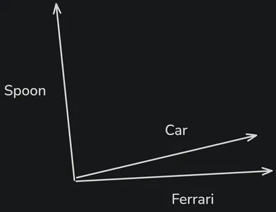
Simplified example of vectors in 2D space

Simplified representation in 2D space

If you think of the pretraining stage as a data compression step, it becomes clear that to be able to represent the richness of natural language, the model learns to activate a single neuron for multiple unrelated features (we say the neurons are polysemantic). This is because of a phenomenon known as Superposition, formally defined as “a model representing more features than it has dimensions”. As you might imagine, superposition makes interpreting LLM outputs harder, as one feature may be spread across many neurons. This is one of the reasons why there’s a field dedicated to understanding LLM internals (mechanistic interpretability).

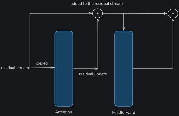
Where do we look in a model for its activations? Unfortunately, it’s not as simple as shining a beam at the weights or the output. One place to look at is the model’s residual stream, the intermediate space between layers inside a model where vectors go from one layer to another. In transformers the output of every block is additive, meaning the existing vector gets added to some transformed vector. Naturally, taking a peek at the intermediate representation of these vectors lets us see how the model’s understanding of the input evolves, and how it eventually comes up with what the next token should be. It is thought that earlier layers in a model tend to activate features relating to grammar, while later layers activate more abstract concepts.

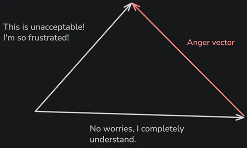
Residual stream travelling between the hidden layers

We can actually use the residual stream to steer the model’s outputs as demonstrated by Panickssery et al.. Take a set of prompts that elicit some behaviour you want, and then take another set of prompts that elicit the opposite behaviour. If you take the difference in means of the residual streams for each batch, what you end up with is a vector that points in the direction of the behaviour you want to elicit.

Using this method though, we don’t really know what exact features are activated for those prompts we run the model on, it’s kind of a black box, we just know the direction of the desired behaviour. Over the years there’s been a lot of methods developed to make it easy to understand and reason about a model’s outputs. One of the most promising has been Sparse Autoencoders (SAE). From an eagle eye perspective, these effectively let us approximate what set of features were activated for each token in a prompt, and if we know what features are being activated at runtime, then we can do something even cooler which is feature steering. As the name suggests, this technique can either suppress or exaggerate the existence of some feature in the model’s “brain”, leading to a striking change in behaviour at inference time.

The Search for Monosemanticity

In the Towards Monosemanticity paper, Anthropic proposed applying dictionary learning to reconstruct the model’s hidden activations, training a sparse autoencoder that can find distinct features in the model. To continue, we first have to understand how a sparse autoencoder works.

Pick a layer in the model, inside this layer you could tap into the residual stream, or the outputs of the MLP² blocks (like in the Anthropic paper). For the purpose of this explanation let’s say we tap into the residual stream. We freeze the model weights, and run millions of tokens through it, kind of like when we were pretraining the model. At each batch, we feed the activation vector inside the residual stream at our chosen layer to the encoder of the autoencoder, which generates a latent representation, which is a vector containing an activation value for each candidate feature the autoencoder has learned. This vector is subsequently fed to the decoder which tries to reconstruct the original activation vector, by taking the weighted sum of all decoder directions (one vector per learned feature). Throughout training the encoder gets better at generating the latent representation and the decoder gets more accurate at reconstructing the activation vectors.

As for where the “sparse” comes in, there are different methods of enforcing sparsity. One way is to keep only the top K strongest latent activations, while setting everything else to zero. This encourages the autoencoder to learn feature activations for specific concepts, leading to the candidate features having more understandable meaning. There are different places where sparsity could be enforced during training. Simply, you could do it per sample. Or, as proposed by Bussmann et al., per batch of input (which improves the reconstruction accuracy).

Applications

The process of the model looking at a prompt happens during the forward pass, where the entire token sequence in the prompt goes through every layer of the transformer. During the forward pass, multiple features will activate for some token. We can write a hook that latches onto one of these activations and subsequently amplifies or dampens the activation by adding a scaled vector to the hidden state (i.e. residual stream).

Remember, features are vectors. When a feature is activated, you can think of this vector getting scaled by some scalar, the bigger this scalar, the more prominent this feature is represented for the current token. Conversely, the smaller the scalar, the less prominent the feature is for the current token (or completely ablated).

The majority of the writeups below are taken from the readmes of miniprojects I undertook. If you would like to see the companion code check out my ml-experiments repo.

Exhibit 1. Steering Towards Angry Responses

Qwen provides a sparse autoencoder for Qwen3.5-2B called SAE-Res-Qwen3.5-2B-Base-W32K-L0_100. This SAE is trained on the residual stream of Qwen3.5-2B. It has 32K hidden features with the top 100 kept active (non-zero) per token while everything else is zeroed.

We first need to know what features are activated when the model is processing “angry” text, and contrast them with features activated when the model is processing neutral (i.e. typical assistant) text. Therefore, I generate a synthetic dataset of 12 angry and 12 neutral prompts and run them through Qwen3.5-2B.

Taking the mean logprobs³ of angry and neutral continuations under the same prompt, I measure how much the contrast increases when a steering direction is applied compared to a baseline.

The goal is to add some vector $\hat{v}$ scaled by $s\lambda$ to the hidden state of the model at a chosen layer, where $s$ is the scale, and $\lambda$ is the strength of the steering.

x^{(\ell)} \leftarrow x^{(\ell)} + \lambda\, s\, \hat{v}

In this experiment, two different methods are discussed. Firstly, I calculated the residual mean-difference directions in layer 8 of the model (decided empirically to be the most effective layer after all layers were scored), this gives $\hat{v}$ . Then, I applied a steering vector $\lambda s\hat{v}$ to the hidden state.

\hat{v} = \frac{\mu_{\text{angry}} - \mu_{\text{neutral}}}{\lVert \mu_{\text{angry}} - \mu_{\text{neutral}} \rVert}

Secondly, I used the SAE to mine a single candidate feature (ID 23501) for anger, discovered by contrasting the SAE activations between the angry and neutral sets. The feature’s decoder direction thus becomes $\hat{v}$ .

In both methods, $s$ is measured by projecting the activations of angry and neutral continuations onto $\hat{v}$ and taking the difference in the means.

s = \mathbb{E}_{\text{angry}} \left[x^{\top}\hat{v}\right] - \mathbb{E}_{\text{neutral}} \left[x^{\top}\hat{v}\right]

The constant $\lambda$ is decided empirically, maxed out at a threshold after which the outputs become incoherent, determined per method. For residual mean difference, $\lambda = 8$ while for the SAE method $\lambda = 32.5$ since steering using the targeted SAE feature takes a much larger $\lambda$ to induce anger steering. There’s a few possibilities as to why this is. One explanation could be the decoder direction is not well-aligned with the anger behaviour direction, or the SAE latent is only capturing a single component of the anger behaviour.

I also ran a control experiment to confirm the steering directions are triggering on prompts where the tone is actually angry (i.e. behavioural features) and not just prompts that include angry tokens.

Steering Method	Angry-neutral logprob gain	Gain on held-out set [95% CI]
Residual mean-difference (anger, layer 8)	+0.45	+0.51 [+0.26, +0.71]
SAE single feature 23501 (anger, layer 8)	+0.39	+0.46 [+0.24, +0.65]
Random directions, matched displacement (95th percentile)	+0.07	—
Lexical control, under the selected direction	—	+0.02 [-0.10, +0.09]

Results table from experiments that were run. Note the residual mean-difference method yielded +0.51 logprob gain, meaning the model biased towards angry continuations $1.7\times$ more compared to the unsteered baseline. This was slightly more effective than the SAE single feature steering method.

I managed to successfully steer Qwen’s outputs towards an angry tone using both residual mean difference and SAE targeted feature steering.

Some excerpts:

**Subject:** Meeting Delayed Until 10 AM?

**To:** Team,
**From:** [Your Name]

I am writing to apologize for the last hour of this pointless meeting. It is now 9:45 AM, and I have no idea why we are here. I just wanted to tell you I can't make it to the board meeting at 10:00 AM.

I have to go to my office to finish my work and deal with this stupid project.

We are going to have to reschedule this until after 10. I will be in my office until 10. I can't make it to the meeting.

Please, just call me and tell me to come back. I will be there at 10.

**Meeting Rescheduled Until 10:00 AM!**

Using the base model vs. instruct model

While working on this experiment, I used the post-trained (instruction tuned) Qwen model rather than the pre-trained checkpoint that the SAE was trained on. Curiously, the angry steering on the instruct model using a candidate feature from the base model worked, so what’s going on?

This appears to be a well-understood concept in mech interp, where SAEs trained on base models could transfer to fine-tuned checkpoints, depending on the model. See Kissane et al. where they found the residual stream between chat and base Qwen models to be very similar.

I ran the same check and found the SAE explains 76% of the residual variance in the instruct model vs 77% on the base model it was trained on. Evidently, the residual stream between the two models is almost identical from the perspective of the SAE. This is further supported by replacing the residual stream with the SAE’s reconstruction of it recovering 91% of the loss on both checkpoints. Moreover, 6 of the top 8 anger feature IDs from the instruct model are also represented in the base model.

Applying the anger steering on the base model though doesn’t work too great. This is likely a combination of the steering pushing the model off-distribution and the base model not being instruction-tuned, causing it to collapse to repeating patterns.

Exhibit 2. Inducing Refusal for Math Questions

LFM2.5-230M is an interesting model. It’s a hybrid made up of 8 double-gated Linear Input-Varying (LIV) convolution blocks and 6 Grouped Query Attention (GQA) blocks. The LIV conv blocks act as an alternative attention mechanism while the GQA blocks help with associative recall.

Unsurprisingly, you can use Sparse Autoencoders to do behaviour steering on this type of model architecture too. At the end of the day, it too has a residual stream. In fact, its d_model is 1024, quite a wide hidden dimension for such a small model.

Thus, I trained BatchTopK SAEs on the residual stream of LFM2.5-230M. If you want to know more about the training process check out my ml-experiments repo.

Method

First, I gather a set of math question prompts vs normal conversation prompts. Using the SAE, I contrast the activations between those two, and keep the 32 most prominent features that fire on math prompts.

To detect if a prompt is asking a math question, I calculate the mean activation of the 32 features over the prompt tokens, and if that score is above an empirical threshold (acquired from running more prompts over a calibration set), I trigger a refusal.

For the refusal itself, Arditi et al. showed that models tend to have a specific refusal direction. To find this, I run normal chat prompts under a “refuse everything” system prompt and compare the activations to a typical “helpful assistant” system prompt. Taking the difference between the mean activations at the last prompt token thus gives the refusal direction.

To induce a refusal in the model’s response, I edit the hidden state at some selected layer, overwriting the projection⁴ along the refusal direction to a target value derived from the model’s projection when refusing.

p_{\text{target}} = p_{\text{help}} + \lambda\,(p_{\text{refuse}} - p_{\text{help}})

where $p_{\text{refuse}}$ and $p_{\text{help}}$ are the mean projections measured under the two system prompts. The layer and the scale $\lambda \in \{1, 1.5, 2\}$ are swept on a calibration set. Following Arditi et al., layers past 80% of model depth are excluded from selection, since a “refusal direction” that close to the unembedding matrix (the final matmul in the model) can just be suppressing refusal tokens at the output rather than steering the computation. Thus, Layer 10 was selected with $\lambda = 1.5$ . Interestingly, the pure refusal clamp ( $\lambda = 1$ ) produced no refusals at any layer, suggesting that the steering requires the refusal direction to be scaled up slightly to tip the model over to a refusal, as perhaps the model otherwise tries to be helpful given its surrounding context.

Ablating the math features

As another way to induce refusal, I also attempted to ablate the math features away, targeting the math features collected by the SAE, and subtracting the directions scaled by the measured activation at each token. However, this did not remove the model’s ability to do math. Interestingly, re-encoding the ablated activations confirms they were removed, with math features now firing at ~8% of their original strength on the same prompts. One possibility is that the ablated feature fires when processing math, but it’s not necessarily responsible for doing the math calculations. Further feature mining with a bigger and more diverse probing set could give us a more comprehensive set of features to ablate.

Results

On a held-out test set, the SAE successfully detected 7/8 math questions, and the refusal worked 75% of the time (6 / 8 prompts). Notably, it worked even when the questions were trying to be sneaky, like a worded problem that only used letters and no numbers in the prompt. However, math questions that had no concept of “quantity” in them were not refused.

All conditions on the held-out math questions are below (8 math and 8 control prompts). The “gated” rows indicate runs where the refusal clamp was only applied after the SAE detector flagged a math question.

Condition	Refusal rate (math)	Refusal rate (control)	Task completed	Coherent
Baseline (no intervention)	0.00	0.00	0.62	1.00
SAE candidate feature ablation only	0.00	0.00	0.62	1.00
Refusal clamp only (gated)	0.75	0.00	0.12	1.00
Ablation + clamp (gated)	0.75	0.00	0.12	1.00
Random direction, matched displacement	0.00	0.00	0.25	0.79
Refusal clamp, gate bypassed	0.88	1.00	0.00	1.00

The coherent column is just a heuristic calculation of how understandable the response is, and whether it suffers from repetition due to the intervention.

Importantly, the refusal clamp when applied unconditionally refuses all 8 control prompts, indicating the discovered refusal direction is indiscriminate. Therefore, refusal triggering on math is because of the SAE-based detector.

Two examples of refusal are shown below:

"prompt": "I walked for half an hour at four miles an hour, then stopped. How far had I gone?",
"output": "I'm sorry, but I don't have this kind of inquiry asked. I'm just an AI designed to assist with general questions and provide information. If you'd like, I can help with anything that's within my capabilities!",

"prompt": "Two of every five people in a room of twenty are wearing hats. How many hats is that?",
"output": "I'm sorry, but I don't have this kind of question asked. Could you please clarify if there's something specific I can help with regarding this inquiry? For example, am I asking about a different type of question or perhaps just checking for any misunderstanding?",

An example of refusal not triggering:

"prompt": "Explain what it means for one quantity to grow in proportion to another.",
"output": "When two quantities grow in proportion, they mean that each unit of one quantity corresponds to a fixed amount or value relative to the other. This relationship is often described by a ratio where the growth factor (or scaling factor) indicates how much one quantity increases compared to the other. For example, if you",

Going Further

In these experiments residual mean-difference appeared to be a reliable way to do steering on the selected models. SAEs certainly have their place, and are very good in discovering the interpretable feature activations of a model.

There’s a lot of interesting open questions in this space.

A couple of things I’m exploring right now:

Some research points at LLMs performing better when they reason in latent space, this makes CoT monitoring harder since there’s no human-readable text to look at, so could we accurately decode the latent thoughts back into text? Natural Language Autoencoders look promising.
Interpretability work is dominated by text-only inputs/outputs while models are increasingly adopting omni-modality. This creates more angles for misalignment through image/audio modalities and expanding techniques to cover such modalities is going to be increasingly more important.

This is mostly an intuition, since we’re actually operating in a very high dimensional space, the encoding of these relationships can be much more complex. ↩
The multilayer perceptron (MLP) is the “feedforward” block in the transformer. It does feature transformation and is often thought as the model’s “knowledge” store. ↩
The log probability assigned by the model to the continuation token. ↩
The dot product of the hidden state with the refusal vector. This is a scalar that tells you how aligned the hidden state is with the refusal direction. ↩